Iterated Prisoner's Dilemma Round 2: Zero Determinant Strategies and Evolving Populations

Last time, we looked at some simple strategies and ran a round robin tournament similar to how Axelrod played out. This time things will get a bit more messy. If you're unfamiliar with iterated prisoner's dilemma, I'd recommend reading the previous post for an introduction to the topic.
Markov Chains and Stochastic Iterated Prisoner's Dilemma
For starters, the strategies considered will be of a more probabilistic form. Given the moves played last round, there is some corresponding probability of cooperating. For player 1, we'll use P={pcc, pcd, pdc, pdd} where pij refers to the probability of cooperating when player 1 played i last round and player 2 played j. For player 2, we similarly define Q. For example, if both players played defect in the previous round, there would be a probability pdd that player 1 cooperates and (1-pdd) that player 1 defects. This is similarly true for player 2.
The transitions between previous moves to new moves can be described with a Markov chain. A Markov chain is essentially a state machine where the weights are permitted to be probabilities of a given transition occurring. A diagram of the states permitted and their transitions is shown below.
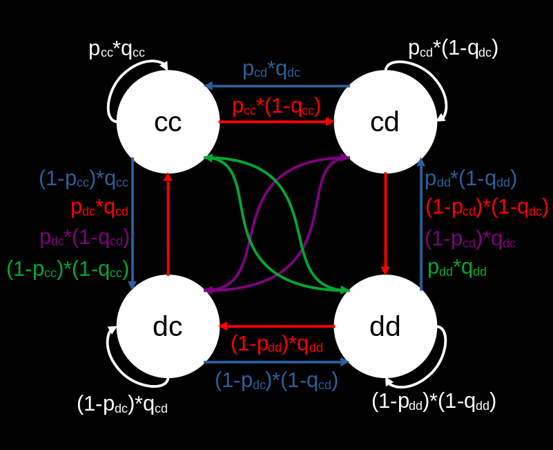
This corresponds to the following transition matrix.

One useful thing with Markov chains is that it can be presumed that a steady state distribution can be achieved over many runs. This means that it's possible to solve an equation of the form v=vM. The vector v defines the distribution of states present as t goes to infinity. This is quite useful as it allows us to determine the end state without taking the time to simulate it all. Acknowledging this to be the case, we will simulate it all anyway as an exercise.
Longer Memories Don't Help
Before we run simulations and analysis, some motivation. One of the relatively recent developments in the study of Prisoner's Dilemma is the set of Zero Determinant Strategies. These strategies use the construction applied here of defining a strategy by a vector transition probabilities dependent on last round. The game when using this construction is called Stochastic Iterated Prisoner's Dilemma. ZDS involves additional constraints on this vector of probabilities which will be discussed later. The reason for only considering the previous round is that it turns out no advantage is conferred through having a longer memory than the opponent. This is unintuitive so the math is shown below.
Let X and Y be random variables that give values x and y which represent the moves of each player. As it stands here, the scores of each round will be entirely determined by the moves selected. By viewing the average of the joint probabilities of x and y over the possible histories of the game, scores can be found. H0 will refer to a shorter memory and H1 will refer to a memory that remembers further back. Calculating the expectation value of this joint probability, this gives the following formula.
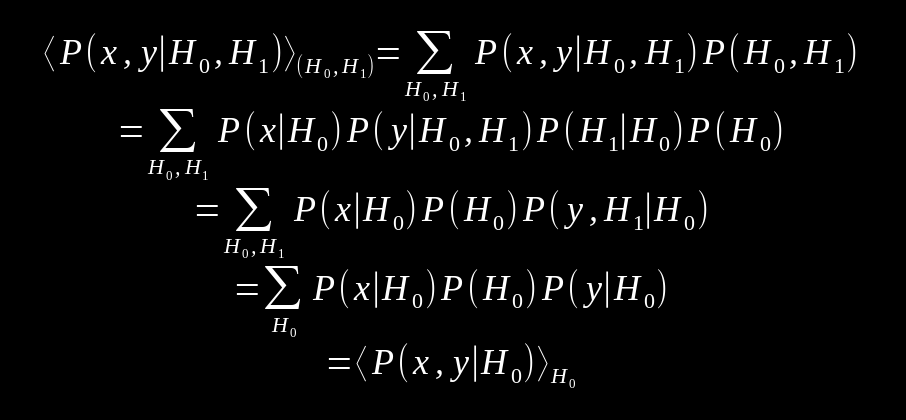
By using the independence of x from H1 and expanding further, we move to the second line. From here the terms are grouped by H0 and H1. In the 3rd to 4th line, the sum over H1 is used on the P(y, H1|H0). Bringing everything together, we get our result.
This can be read as the joint distribution of x and y given histories H0 and H1 is equivalent to the distribution wherein H1 is H0. Turns out that a longer memory does not help when simply considering previous moves. In the paper, it's described that a longer memory does not help unless a "theory of mind" applied to the opponent is included. This is connected to the strategies being independent of their opponent's score.
Zero Determinant Strategies
Now knowing that longer memories do not help, it's reasonable to use the Markov model shown to examine our game. Through a series of manipulations, the relation below is found.
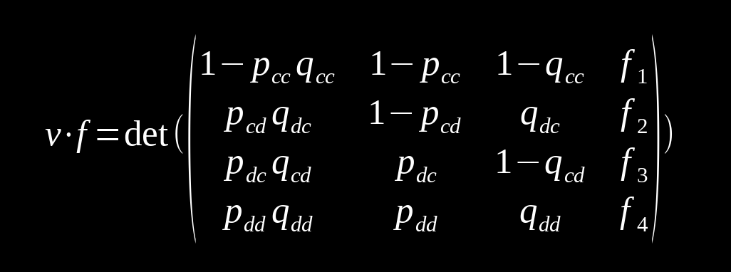
A nice property gained from these manipulations is that columns 2 is determined entirely by p and column 3 entirely by q. Here we'll denote these vectors as ps and qs In this way we can write D(ps, qs, f) as a shorthand for this determinant. This comes in handy because if we define SX=(R, S, T, P) and SY=(R, T, S, P), we can find the scores for each player from the stationary distribution v with the following formula, replacing x with y for player 2's payoffs.
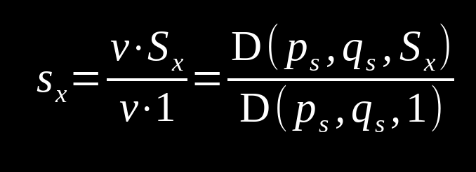
Because these scores sx, sy are linear with respect to the payoffs, we can write a linear combination of scores.

By choosing ps or qs such that they create linear dependence on f, it can be assured that this determinant is equal to zero. This in turn allows for a linear relationship between the player's scores. Strategies that enforce the condition of zero determinant are called zero determinant strategies (ZDS).
From this, by choosing one player's probabilities, a few situations can be chosen. A player employing this strategy may set the score of their opponent or extract an extortionate share from them. Details on this are found in the paper by William Press and Freeman Dyson cited below.
One case of note is that when employing an extortionate strategy with minimal extortion, the strategy ends up reducing to our well known tit for tat strategy, corresponding to the v=(1,0,1,0). So tit for tat is actually a zero determinant strategy! One thing that this model shows though is that linking one's score to the other's does not necessarily end up in the symmetric payoffs found in tit for tat. It may be possible to manipulate another player in order to get an extortionate share.
Simulation Time!
Rather than examine the raw analytic form of ZDS, we look at the stochastic iterated prisoner's dilemma naively. A population of players is generated for the whole probability space in steps of 0.09. This ends up with around 20k players. For each generation, the players are randomly matched up and play each other. Upon completion of play, the winner is copied and the loser dies. This is done for 50 generations. By the end of this, most of these simulations converge to a singular winner.
Simulations were run on a laptop for a few days, with the probability vector of each player being saved off in every generation. The distribution of probabilities from all the player's strategies over time is shown below as an example.
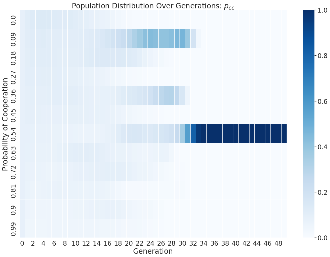
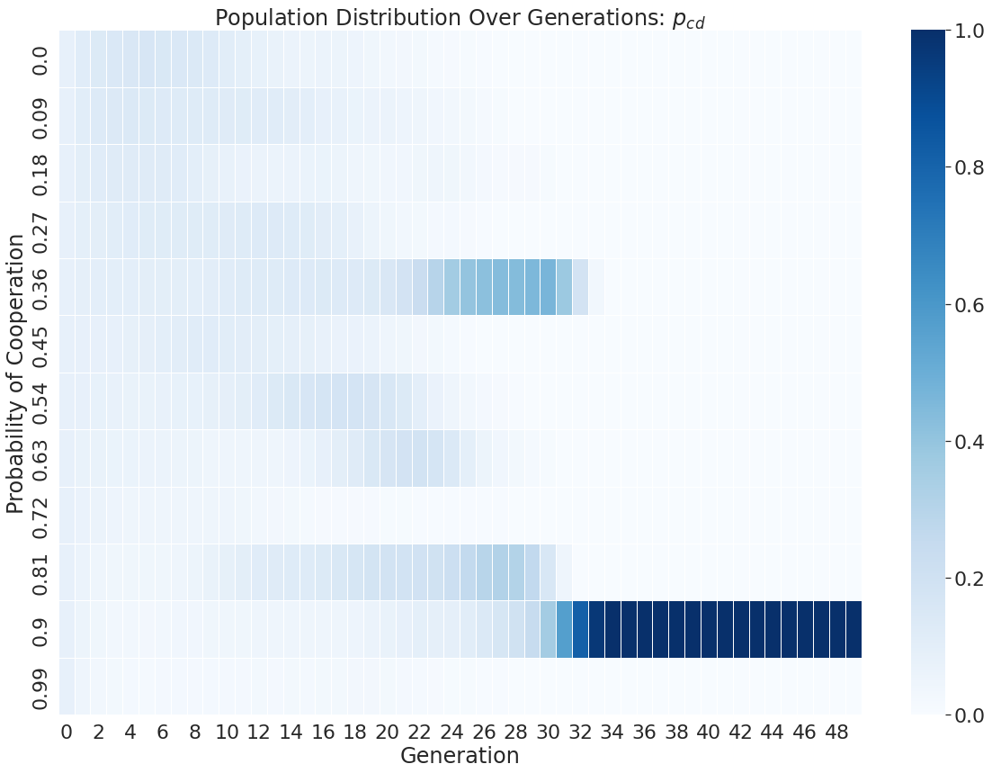

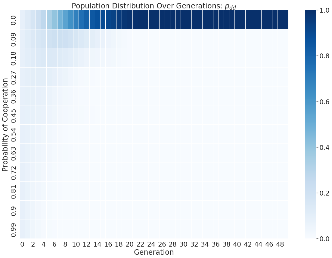
In this particular run of the evolution, we see that pdc and pdd converge to zero, meaning always defect when defected previously. We also see pcc go to a 54% change of cooperating and pcd goes to a 90% change of cooperating.
The pdc and pdd results are in line with what can be expected from some viable strategy of ZDS, but overall it seems a single run through evolution may not be that meaningful. Because of this, 1000 instances of this were run to build statistics for the following analysis.
Analysis
Because these simulations were simply run for some number of iterations, there is no assurance that a single unique probability vectors remains at the end. Fortunately, we can weigh each probability vector by their populations for following analysis.
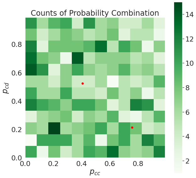
Some traits worth considering are what strategies actually end up being viable by the end. Initially only 98 runs of this simulation were performed. A few strategies ended up being more viable than others but not by a clear margin. Following up, 1000 more runs were performed. Shown below is the population of each unique strategy that remained to the end.
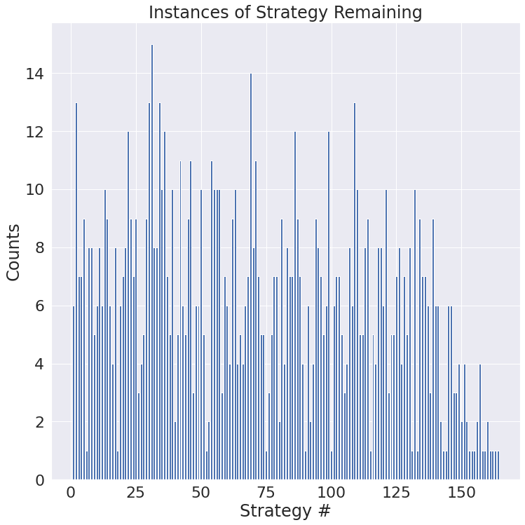
From the looks of it, if the simulation itself is running as intended, more compute is required to see a more general convergence. It also may be possible that some of the strategies here are only off from each other by a single step.
Briefly, the red dots are centers for k-means with 2 regions, there doesn't appear to be anything here.
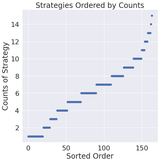
As a passing curiosity, here's the sorted version of converged results. Wouldn't be surprised by some power law lying underneath here but given the poor convergence overall it seems to be a bit of a reach for a concrete statement.
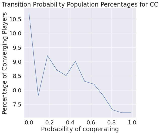
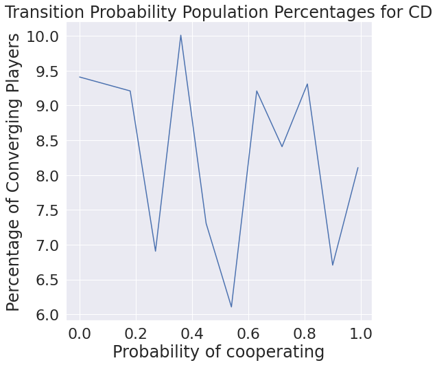
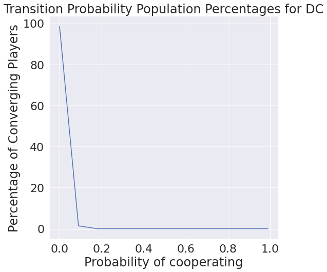
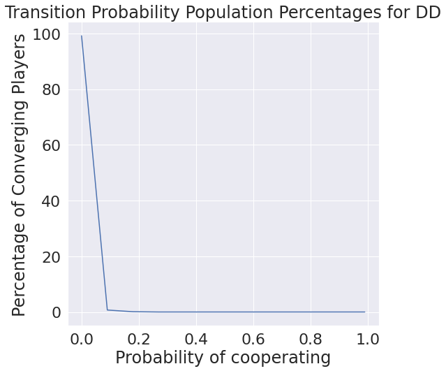
Only considering what we have though, it may be interesting to see the distribution of each probability of transition. We find that cooperating after mutual defection is basically never chosen, which makes intuitive sense.
Next Steps
It seems it is necessary to get additional compute to be able to perform these simulations in a timely fashion. Another option would be to choose evolution schemes that converge quickly and to include a convergence check in the actual runs. This would ensure no compute is spent on rounds that are not determining anything new. While this would be good, for now we'll move on to propose a new approach to the game in the next entry in this series.
Materials
Continuing on with Rust for this project in general. Given the sheer number of players, the simple multithreading approach is growing strained. It is likely that soon enough a threadpool will prove beneficial for running more rounds without hitting stackoverflow.
Transitioning the data storage setup to something like mongoDB would be a positive improvement although it's unclear how necessary that is for a homebrew project like this.
Once again, the analysis on the data generated from Rust was performed in python. Nothing fancy, just bar graphs over populations and distributions of probabilities. Might be worth it to try out some of this with Rust, but jupyter notebooks are convenient.